Fake Coffee with a Known Answer
This series has measured Gagné's example photo many times without ever checking whether the numbers are right. I made fake photos in which every particle's size is known, tuned them to the real photo's blur, uneven lighting, noise and shapes, and graded the series' measuring algorithm. A volume-median error of 6% on smooth fakes became 33% on real-like fakes, and most of it came from touching particles caught as one blob.
So far this series has measured one photo, Gagné's example picture, many times over. I set the scale with a coin, flattened the background, cut out the particles, gave them diameters, and counted them by number and by volume. The median circle-equivalent diameter of 1,572 particles came out at 605 µm. But I never checked whether that number is right. Nobody knows the true size of the particles in that photo.
Last time I pushed virtual grounds of known size through a sieve, a laser and a camera to compare the instruments. This time I grade the camera's algorithm itself. I make fake photos in which I know the size of every particle, measure them with the method this series has been using, and compare the result with the answer.
A photo has no answer key
To grade an algorithm you need the right answer. With a real photo, two ways come to mind: have a person trace every particle, or measure the same grounds with another instrument.
Both are shakier than they sound. Hand-drawn outlines differ from person to person. Rühle and colleagues (2021), working with electron-microscope particle images, reported that their ground-truth masks and a human operator disagreed by about 9 nm, or 1.2 pixels. In size that is around 5%. Other instruments, as the last post showed, each hold up a different ruler. Tune a photo algorithm to match sieve results and you are training the photo to imitate the sieve.
So other fields build photos with a known answer on purpose. The 1951 US Air Force resolution chart and the slanted-edge targets of ISO 12233 are used to measure camera resolution: the line spacing is known, so blur can be measured exactly. Cell biology has collections of computer-made cell images. The Broad Institute's BBBC005 contains 19,200 simulated images with 1 to 100 cells each, drawn at 48 levels of focus blur. The cell count is in the file name, so a cell-counting algorithm can be graded right away.
Particle sizing does this too. Frei and Kruis (2020) trained a neural network to size agglomerated, partly sintered nanoparticles using only synthetic images, to skip manual labelling and to get better ground truth. Mill and colleagues (2021) rendered nanoparticle microscope images in the 3D graphics program Blender for training, and got almost the same performance (F1 0.930) as training on real images (F1 0.950).
I found no study that grades coffee-grounds measurement this way. Gagné's coffeegrindsize repository has no known-answer test either. So I made one.
Five steps to a fake photo
A fake photo is made in five steps.
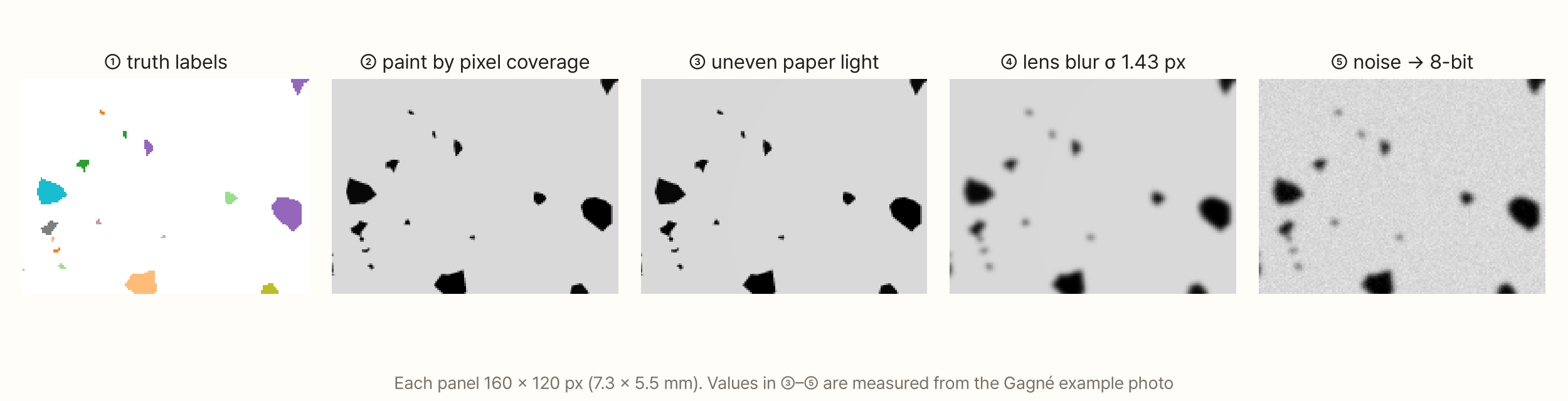
- Decide the answer. Particle sizes are drawn from the bimodal model built in "Count by Number or by Volume." The coarse peak continues the particle distribution measured in Gagné's photo, and the fines peak holds 20% of the mass. When Bora and Briesen (2026) fitted ten mixture distributions to ground coffee, the grounds always had two peaks. Each particle's elongation is picked from the 1,578 values measured in Gagné's photo, and its orientation is random. Particles smaller than 100 µm are barely two pixels at this scale, so they are not drawn
- Paint in pixels. Particles are drawn on a canvas four times larger and then shrunk, so an edge pixel darkens only by the area the particle covers. The large canvas, painted with particle numbers, becomes the truth label
- Add uneven paper brightness. Bright in the middle, darker toward the corners
- Blur with the lens. A Gaussian blur
- Add noise and save as 8-bit
The values for steps 3–5 were measured on Gagné's example photo. Fitting the brightness profile across the edges of 300 large particles gave a blur of σ 1.46 pixels; removing the effect of pixel area leaves a lens blur of σ 1.43 pixels. The darkest paper (bottom 5%) was 74% as bright as the brightest (top 5%). Brightness noise on empty paper far from any particle was 2.4%, and the grounds covered 6.1% of the paper. Inside a particle the blue channel is close to zero. That is why Gagné uses the blue channel: his manual notes that brown has almost no blue in it.
Does the fake look like the real thing?
The first fake looked like this: particles drawn as smooth ellipses, scattered evenly over the paper.
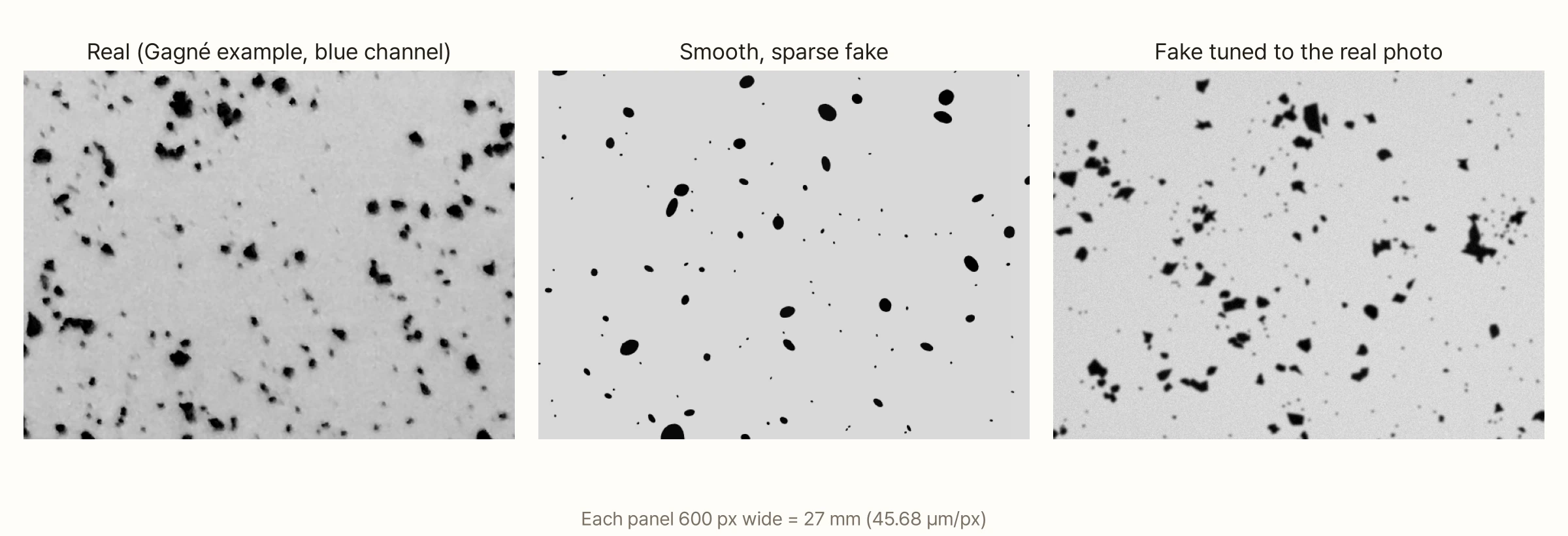
You can see the difference. Real coffee fragments have sharp corners and fall in groups. The fake is too smooth and too even.
Looking alone cannot tell you how close they are, so I measured real and fake with the same method and compared numbers: blob diameter, elongation, solidity (blob area ÷ the area of the smallest convex polygon around it), the share of blobs with solidity below 0.8, and the number of blobs. Blobs with low solidity are usually several particles stuck together.
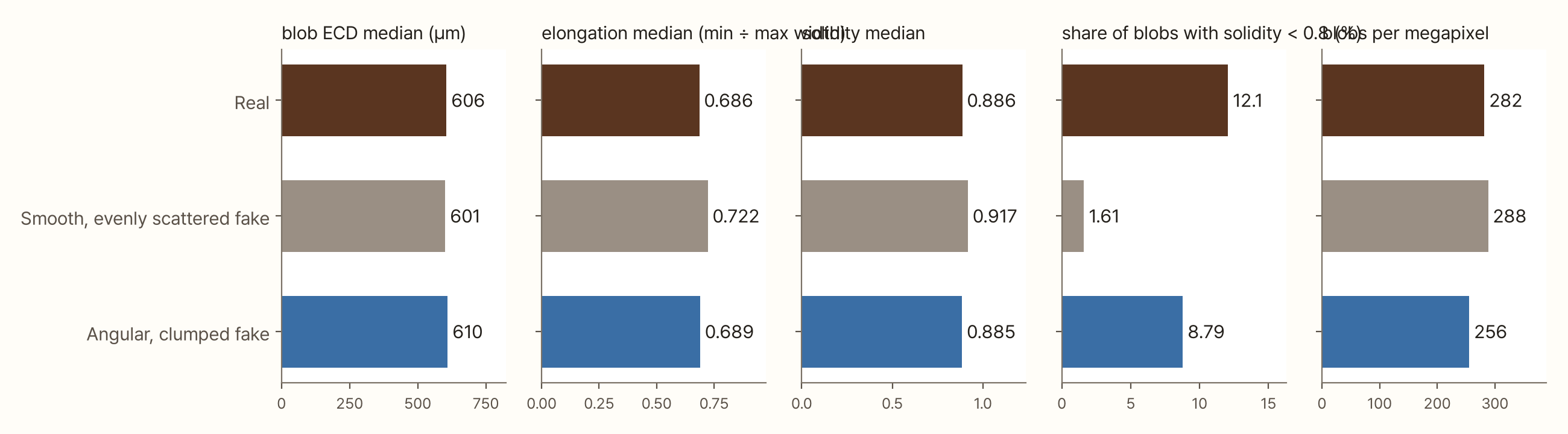
The smooth fake matched the real photo on diameter and blob count but not on shape. Blobs with solidity below 0.8 made up 12.1% in the real photo and only 1.6% in the smooth fake. So I changed the particles into angular shards with 6–10 corners and dropped half of them into clumps about 1 mm across. I tried several values for the angularity and the clump size and kept the one closest to the real photo's statistics. The tuned fake came out at 610 µm diameter, 0.689 elongation and 0.885 solidity, almost the same as the real photo. Its share of low-solidity blobs (8.8%) and its blob count (256) are still a little below the real ones.
There is a reason not to skip this step. Inverse problems have a term for it: the "inverse crime." It describes what happens when the assumptions used to make synthetic data are the same as those used to analyse it, so results look far better than they really are. Colton and Kress, who coined the term, stressed that synthetic data must come from a forward solver with no connection to the inverse solver. In our case: the measuring algorithm expects separate particles, even paper and sharp edges. Build the fakes that way and the algorithm passes easily. There is also a prescription from the opposite direction. "Domain randomization," used in robot learning, does not fit the fake to one real example; it varies conditions so widely that reality looks like just another variation (Tobin and colleagues, 2017). Here I chose to fit one real photo first.
How to grade
The algorithm being graded is exactly the method this series has used. In the blue channel it estimates the brightness of empty paper, flattens the photo, and treats any pixel darker than 58.8% of the paper as particle. 58.8% is coffeegrindsize's default. Touching pixels are grouped into blobs, and blobs under 40 pixels are discarded. At this scale 40 pixels is a diameter of about 330 µm, so grading covers only particles whose true diameter is 330 µm or more.
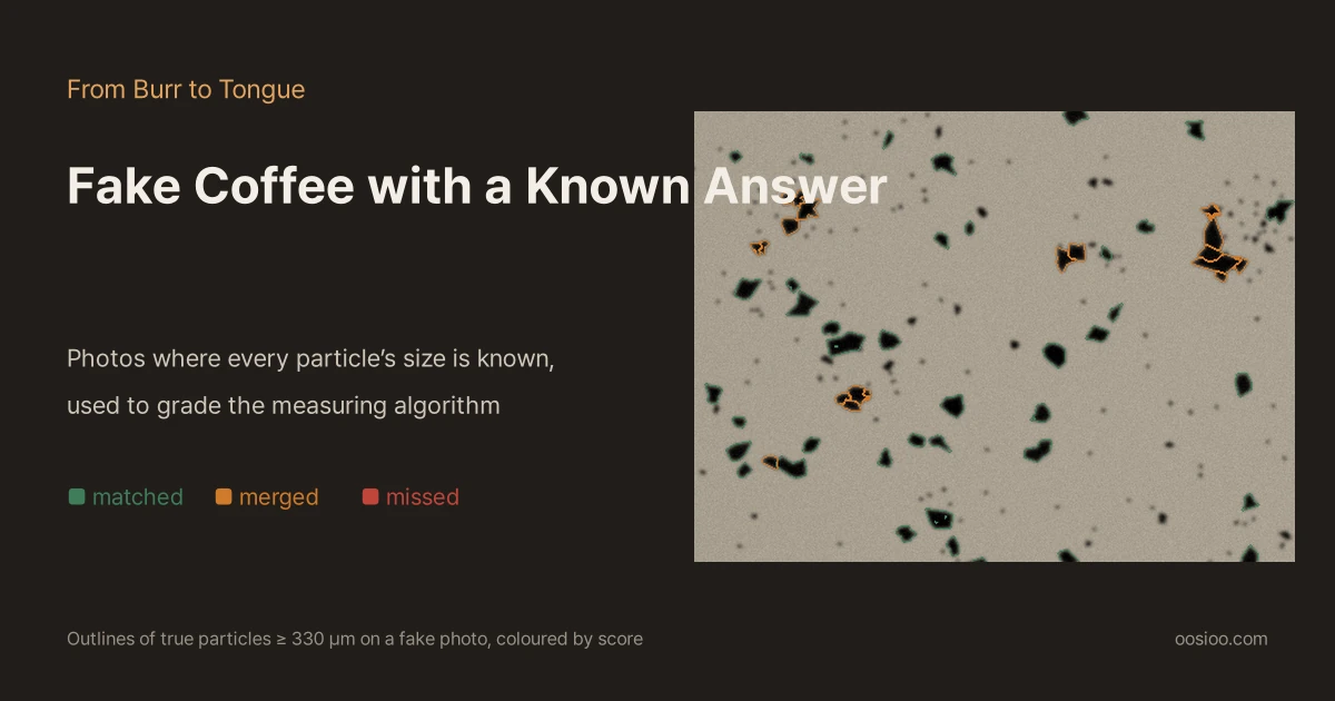
For each particle I check how much its true region overlaps a measured blob. If the overlap area divided by the combined area (IoU) is 0.5 or more, it is "matched." This is the criterion the object-detection challenge PASCAL VOC used to count a detection as correct. If a blob covers more than half of the true particle but the IoU is below 0.5, the particle was caught in one blob with its neighbours, so it is "merged." If no blob covers half of it, it is "missed."
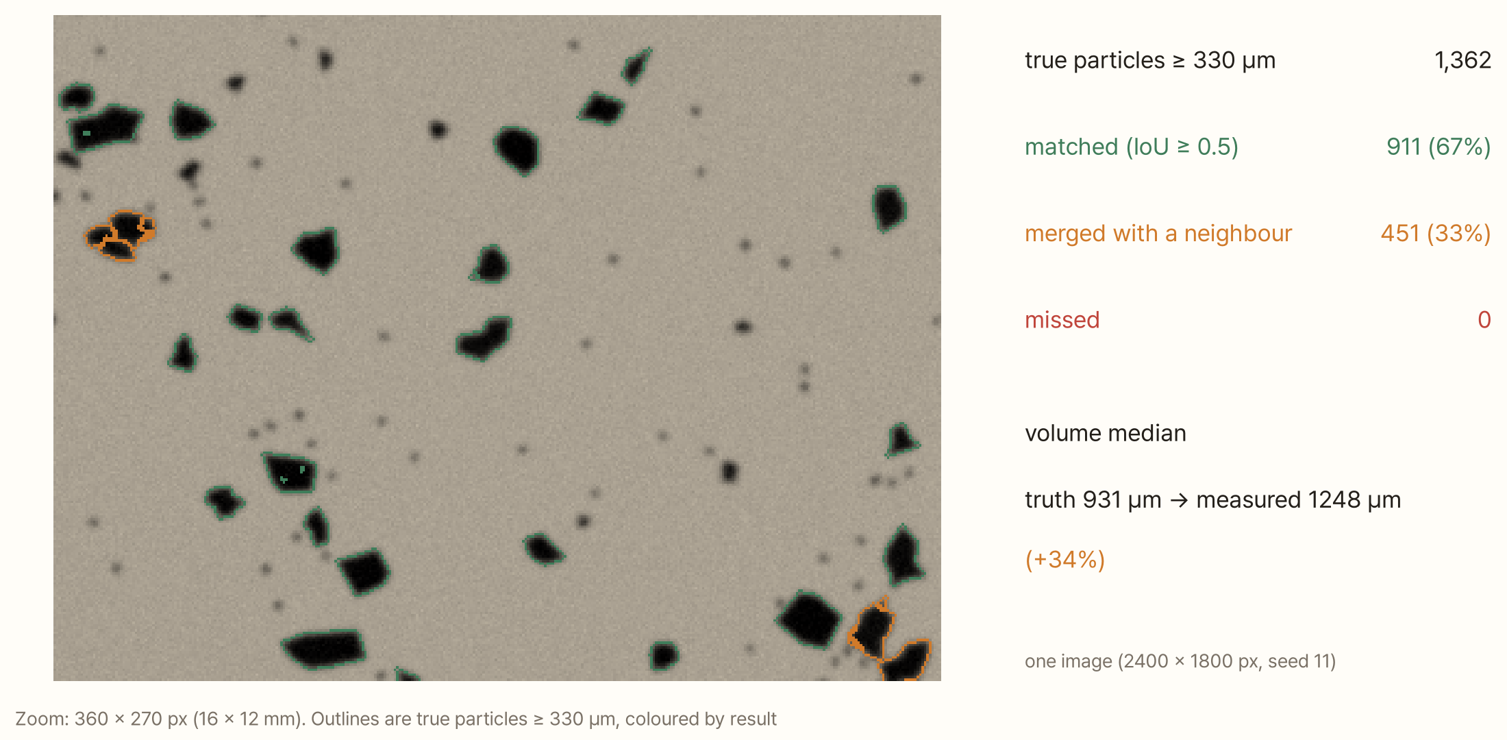
Averaged over three real-like fake photos:
| Smooth, sparse fake | Real-like fake | |
|---|---|---|
| Large particles matched | 95% | 70% |
| Large particles merged | 5% | 30% |
| Large particles missed | 0% | 0% |
| Size bias of matched particles | +2.7% | +6.2% |
| Number-median error | +0.8% | +8.0% |
| Volume-median error | +5.7% | +33% |
Graded only on the smooth, sparse fake, this algorithm is a star pupil. It gets the number median within 1% and the volume median within 6%. On the real-like fake the volume median comes out 33% too large. Same algorithm, different exam, different score.
Nothing was missed: at this resolution every particle of 330 µm or more is visible. Almost all of the error comes from merging. When two or three touching particles are caught as one blob, a single particle 1.4–1.7 times wider appears. Volume goes with the cube of diameter, so these fake large particles push the volume distribution up sharply.
What causes the error
I repeated the same grading while changing one condition at a time. Everything else stayed at the real-like fake, and each point averages three photos with different random seeds.
How densely the grounds are spread
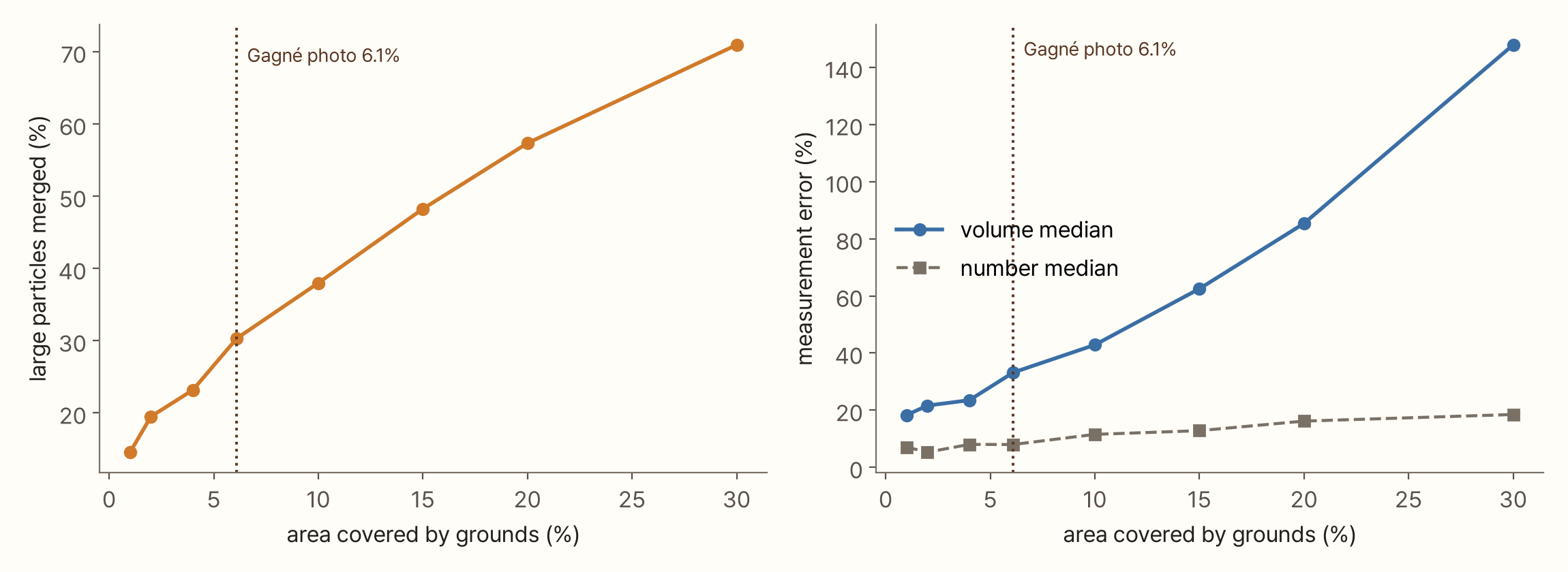
The more sparsely you spread the grounds, the less merging. Spread as densely as Gagné's photo (6.1%) and 30% of large particles merge, putting the volume median 33% too high. Cover 30% of the paper and seven in ten large particles merge, and the volume median is 2.5 times too large.
Look at the left end. Even spread so thinly that only 1% of the paper is covered, 15% still merge, because the grounds fall in clumps. The evenly scattered smooth fake merged only 5% at 2% coverage. Spreading thinly is not enough; clumps have to be broken up.
The international standard for static image analysis, ISO 13322-1, puts this first: "It is a prime requirement of the method that measurements shall be made on isolated particles. Touching particles measured as one particle without a proper separation will introduce error." It goes on to say that touching particles often cannot be detected reliably by image analysis alone, so their influence should be checked experimentally by increasing or decreasing the number of particles per image. The chart above is exactly that experiment. Gagné's manual also asks for particles to be separated by about 5 pixels.
The bias built into the threshold
Even in the clean case with no merging, matched particles came out 2.7% too large. The cause is the 58.8% threshold. An edge pixel half covered by a particle has about 50% of the paper's brightness. That is darker than 58.8%, so it counts as particle. Working it through, a pixel counts as particle once the particle covers 41% of it. Area is effectively rounded up rather than rounded, so particles grow slightly.
Blur makes this bias larger. Across a blurred edge, brightness rises gradually from particle to paper. Because the threshold sits above the midpoint (50%), the place where brightness crosses it is pushed outward from the particle, by 0.22σ for a Gaussian blur. At the blur of Gagné's photo (σ 1.43 pixels) each edge moves out about 0.3 pixels, so a particle 13 pixels (600 µm) across grows by about 5%. The grading found a bias of 6.2%.
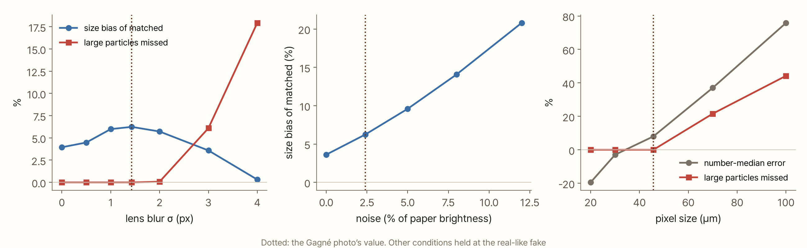
With heavier blur (σ 3 pixels or more), small particles start to vanish: blurred out, even their darkest point no longer reaches the threshold. At σ 4 pixels, 18% of particles of 330 µm or more are missed. This is also why the bias curve comes back down: the small particles that were measured too large drop out entirely, so the remaining particles look less biased.
Noise mattered more than I expected. With noise at 12% of paper brightness, matched particles came out 21% too large. Paper pixels near an edge that happen to dip below the threshold because of noise get attached to the particle.
Resolution behaves as in "The Size of a Single Pixel." Photograph the same scene at 70 µm per pixel and the 40-pixel floor becomes a 500 µm diameter, missing 22% of particles of 330 µm or more. Go the other way to 20 µm and the number median comes out 20% small. That is less an error than a matter of definition: particles smaller than 330 µm become visible, so the median drops below that of the answer, which counts only particles of 330 µm or more. With the same algorithm, changing the resolution changes what is being counted.
Trying fixes
With an answer key, you can measure the effect of a fix too. I tested three.
- Lower the threshold to 0.5. Only pixels more than half covered count
- Split touching particles. Place a seed wherever the distance from the blob edge forms a peak, and divide the blob with the watershed method, a common technique in image analysis
- Drop blobs with solidity below 0.85. Blobs that look like stuck-together particles are not counted at all. This is the filter used for shape statistics in "What Is a Diameter?"
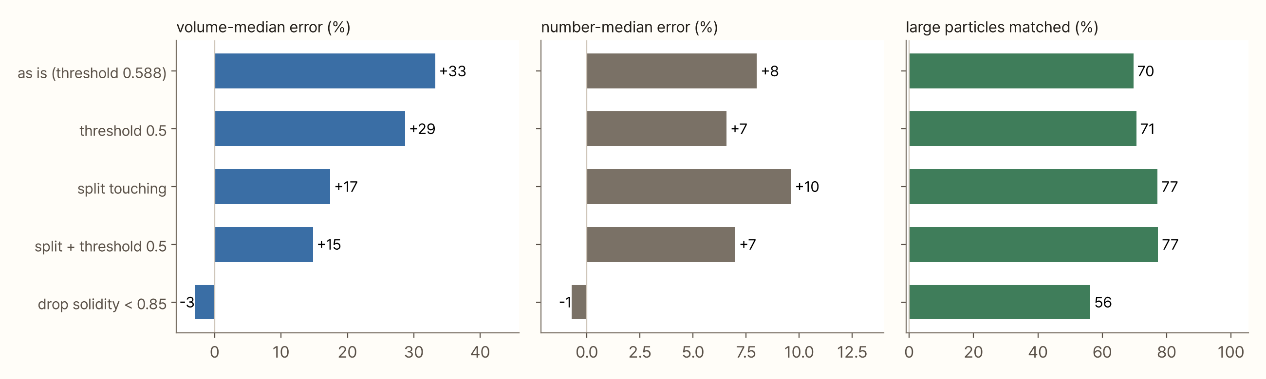
Lowering the threshold to 0.5 removes the size bias of matched particles, from +6.2% to −0.2%. But the volume-median error only drops from 33% to 29%, because most of the error comes from merging, not bias.
Splitting touching particles halves the volume-median error to +17%, and with the 0.5 threshold it reaches +15%. Even so, 21% of large particles stay merged. When angular shards overlap, the distance map often has a single peak, and there is nowhere to split.
Filtering by solidity gives the best-looking numbers: −3% on the volume median and −1% on the number median. In exchange it throws away 44% of the large particles. If the discarded blobs were picked evenly regardless of size, the distribution of what remains would be unchanged, and you would simply take more photos to make up the loss. The catch is that larger particles touch their neighbours more easily, so more of the large ones are discarded. That is why the error is −3% and not zero.
This is where the inverse crime comes back. These fakes were tuned to the real photo's solidity statistics. It is no great surprise that a solidity filter works well on them. To claim it works as well on real coffee, you would need to check that fake and real also agree on properties unrelated to solidity.
coffeegrindsize also has a feature that breaks up stuck-together blobs, using the brightness change near their edges. Comments left in the code show that its key value was changed from version to version, from 0.07 to 0.2 and then to 0.35. 0.07 was "too agressive," and 0.35 "seems much better on Lido and Forte images." It was tuned by eye on photos from two grinders. With photos of known answer, that value could have been chosen by the numbers.
Try it yourself
In the simulation below you can make fake photos and grade them yourself. The photo is 720 × 540 pixels, smaller than in the article, so it holds only a hundred or so large particles and the numbers wobble from photo to photo. Press "Sprinkle again" a few times to see that wobble.
Press "Smooth, sparse fake" and the score is nearly perfect; go back to "Real-like fake" and the orange outlines multiply. Try turning clumping down to 0 or changing the coverage. "Measure the real photo" measures a same-sized part of Gagné's photo with the same algorithm. A real photo has no answer key, so you only see the measurement.
What this experiment leaves out
- The fakes are flat paintings. Real particles are three-dimensional and cast shadows and highlights. Things like shadows or faint rims around particles are not in these fakes
- Fines below 100 µm are not drawn. In real photos such fines darken the paper slightly or cling to coarse particles and widen their outlines
- The clumping is a simple model. Half the particles are dropped at random into clumps about 1 mm across. It does not capture why or how real grounds clump
- The fakes are tuned to the statistics of one real photo. Change that photo's lighting, camera or way of spreading and they would need tuning again. The share of low-solidity blobs and the blob count are still below the real photo's
- Only one algorithm was graded, this series' method. coffeegrindsize's blob breakup and other programs were not graded
- The error on real photos is still unknown. What this post shows is the error on a real-like fake. How wrong the measurement is on real coffee has to be checked against physical objects of known size
Summary
- A real photo has no answer key. Hand-drawn outlines wobble by about 5%, and other instruments hold up different rulers. So I made fake photos in which every particle's size is known and graded the algorithm on them
- The fakes are made in five steps: truth labels → paint by pixel coverage → uneven paper brightness → lens blur → noise. The blur σ 1.43 pixels, 26% brightness variation, 2.4% noise and 6.1% coverage were measured on Gagné's example photo
- Smooth ellipses scattered evenly were far smoother than the real photo. Dropping angular shards in clumps made the diameter, elongation and solidity measured by the same method almost match the real photo
- The volume-median error was +6% on the smooth, sparse fake and +33% on the real-like fake. When the assumptions behind the fakes match the algorithm's own, the score is inflated (the inverse crime)
- Most of the error came from merging, touching particles caught as one blob. 30% of large particles merged, and when grounds fall in clumps 15% merge even with only 1% of the paper covered
- The 58.8% threshold measures particles 2.7–6% too large. Splitting touching particles cuts the volume-median error to +15%; filtering by solidity brings it to −3% but throws away 44% of the large particles
A photo with a known answer is an exam for the algorithm. Check that the exam resembles the real problem before you trust the score.
References
- Rühle B, Krumrey JF, Hodoroaba V-D (2021). Workflow towards automated segmentation of agglomerated, non-spherical particles from electron microscopy images using artificial neural networks. Scientific Reports 11, 4942. doi:10.1038/s41598-021-84287-6 — ground-truth masks vs. a human operator differed by about 9 nm (1.2 px, about 5%)
- Frei M, Kruis FE (2020). Image-based size analysis of agglomerated and partially sintered particles via convolutional neural networks. Powder Technology 360, 324–336. doi:10.1016/j.powtec.2019.10.020 — trained on synthetic images only
- Mill L, et al. (2021). Synthetic Image Rendering Solves Annotation Problem in Deep Learning Nanoparticle Segmentation. Small Methods 5, 2100223. doi:10.1002/smtd.202100223 — F1 0.930 trained on synthetic vs. 0.950 trained on real (SiO₂, arXiv:2011.10505 version)
- Broad Bioimage Benchmark Collection. BBBC005 — 19,200 synthetic cell images, 1–100 cells, 48 focus-blur levels. link
- Lehmussola A, et al. (2007). Computational Framework for Simulating Fluorescence Microscope Images With Cell Populations. IEEE Transactions on Medical Imaging 26(7), 1010–1016. doi:10.1109/TMI.2007.896925
- Bora M, Briesen H (2026). Characterization of Bimodal Particle Size Distribution of Ground Coffee Powder. Journal of Food Process Engineering 49(6), e70645. doi:10.1111/jfpe.70645
- Wirgin A (2004). The inverse crime. arXiv:math-ph/0401050 — definition of the inverse crime; Colton and Kress (1992): synthetic data must be obtained by a forward solver with no connection to the inverse solver
- Kaipio J, Somersalo E (2007). Statistical inverse problems: Discretization, model reduction and inverse crimes. Journal of Computational and Applied Mathematics 198(2), 493–504. doi:10.1016/j.cam.2005.09.027
- Everingham M, et al. (2010). The PASCAL Visual Object Classes (VOC) Challenge. International Journal of Computer Vision 88, 303–338. doi:10.1007/s11263-009-0275-4 — a detection is correct if IoU exceeds 50%
- ISO 13322-1:2014. Particle size analysis — Image analysis methods — Part 1: Static image analysis methods — measuring isolated particles is the prime requirement; vary the number of particles to check the influence of touching (§5.2). official sample
- Gagné J. coffeegrindsize. GitHub. link — blue channel, default threshold 58.8%, manual advice to keep particles about 5 px apart, code comments on the blob-breakup value
- Tobin J, et al. (2017). Domain randomization for transferring deep neural networks from simulation to the real world. IROS 2017. arXiv:1703.06907
Image credits
- All figures and the simulation: my own. The real photo is part of the example picture in Jonathan Gagné's coffeegrindsize (MIT licence), and the elongation of the fake particles was also measured on it