A Distribution with Two Peaks

In the last piece we saw that the size distribution of ground coffee has two peaks. The large peak follows the grinder dial, and the fines peak stays near 30–40 µm, the size of a cell inside the bean. A model that breaks a tissue of cells produced the same shape.

This piece is about squeezing that distribution into a few numbers. A laser-diffraction instrument hands you a curve with dozens of bins. To compare grinders or feed an extraction model, you have to reduce that curve to a handful of numbers. Comminution theory already has distributions for the job. The trouble is that most of them have only one peak. I'll look at what gets lost when you fit them to two-peaked coffee grounds, and then whether a two-peak model lets you say exactly how much of the grounds are fines.

The distributions of comminution theory have one peak

The classic way to write a size distribution as a single formula came from powdered coal. In 1933 Rosin and Rammler summarised sieve results for finely ground coal in an empirical formula: the weight fraction R left on a sieve falls with size x like this.

R(x) = exp(−(x / x′)ⁿ)

x′ is the size below which 63.2% of the powder lies. n says how even the distribution is: a large n means sizes bunch up in one place, a small n means they spread out. Mathematically it is the same formula as the Weibull distribution. Weibull arrived at it independently from the statistics of material strength, where a material breaks at its weakest point. It is still the most widely used distribution in comminution theory. The lognormal distribution, which assumes the logarithm of particle size is normally distributed, is also common. Both describe a distribution with two numbers, and both have one peak.

The Rosin–Rammler formula comes with an old trick. Take the logarithm twice and ln(−ln R) becomes a straight line in ln x. So you plot sieve results on 'Rosin–Rammler paper' drawn with this scale, rule a straight line, and its slope is n. Coffee grind studies use this too. Khongphinitbunjong et al. (2025) ground light, medium and dark beans at 12 settings, measured them by laser diffraction, and compared evenness by fitting the Rosin–Rammler formula; according to the abstract the fits had high R². The full paper is paywalled and I could not read it.

Fitting coffee grounds

I tried it on the four powders from Mo et al. (2023) that we saw last time. The raw data aren't public, so I read the four curves in Figure 3 of the paper (CC BY) by colour and turned them into numbers. The volume below 100 µm computed from my readings came out at 29.7%, 26.9%, 20.4% and 9.9%, within 0.6 percentage points of the 29.2%, 27.5%, 20.3% and 9.7% in the paper's table. The Sauter diameter d[3,2] came out at 76–203 µm, about 5% below the paper's 81–214 µm. I put that down to not reading the very small tail fully from the figure. The numbers below carry errors of about this size.

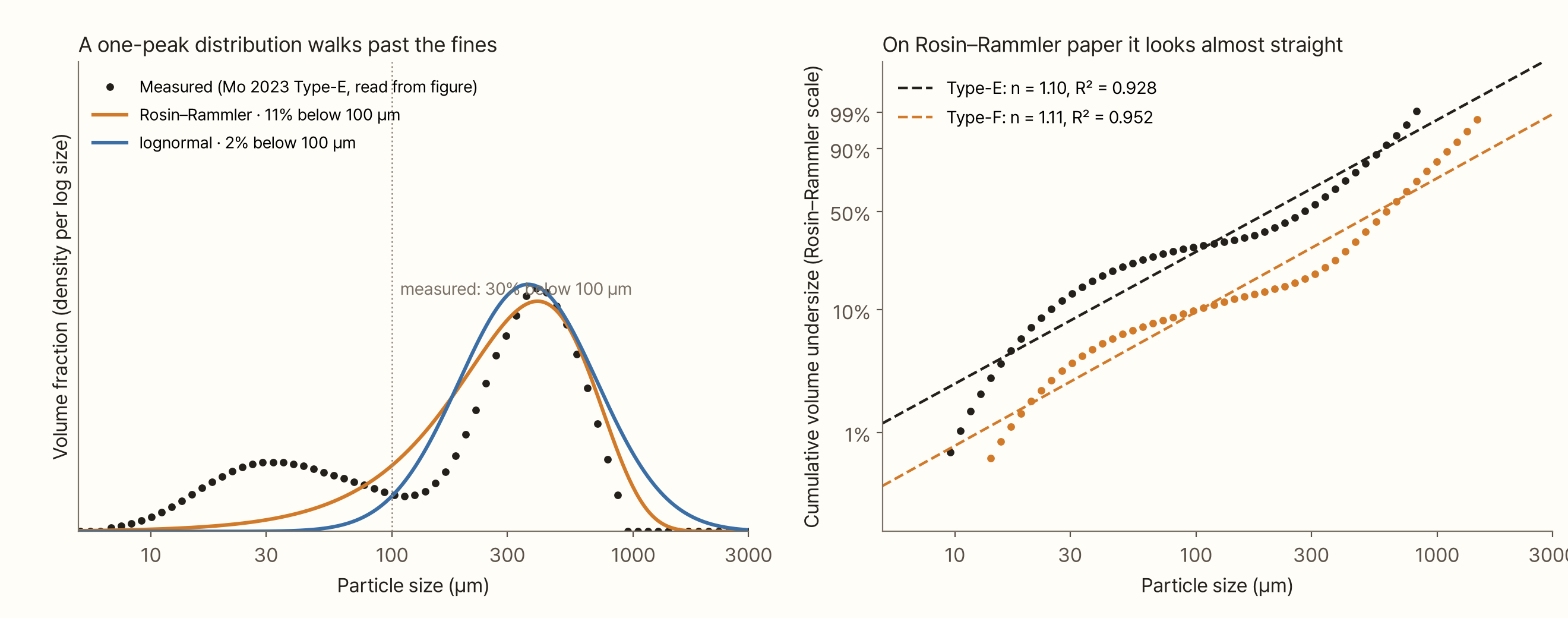
The left graph fits two one-peak distributions to the espresso grind (Type-E). Both curves chase the large peak and walk straight past the fines peak. The measured volume below 100 µm is 30%; Rosin–Rammler gives 11% and lognormal 2%. Rosin–Rammler misses two thirds of the fines, and lognormal misses almost all of them.

The right graph puts the same data on Rosin–Rammler paper. The points bend like a wave. Yet a straight line through them gives R² of 0.93 and 0.95, which looks quite good (0.92–0.95 for all four powders). A cumulative curve rises smoothly by nature, so you can miss a whole peak and R² hardly drops. Judge by R² alone and you'll think the fit is fine.

The evenness number n also depends on how you fit. A straight line on the paper gives n of 1.10–1.14 for all four powders. Fit the density curve directly and n is 1.5–2.0. In the straight-line fit, the points on the fines side tilt the slope down. The 'evenness' of the same powder changes by almost a factor of two with the method, so before comparing your n with another paper's, check how they fitted it.

Why two peaks

Mineral comminution has its own explanation for a distribution that splits in two: particles break in more than one way. When a particle splits into a few pieces, the pieces scale with the original size. When its surface wears away, you are left with a body close to the original size plus very fine dust. In simulations of crushed rock inside a fault, splitting spread the distribution out, while abrasion piled the fine dust up separately and produced two peaks (Mair and Abe 2011). Grinding process models write the distribution of pieces from a single break as the sum of two power laws, Austin-style, with one of the two terms carrying the share of fine pieces (Petrakis 2023).

I couldn't find an experiment that settles whether coffee fines come from wear at the burr surface or from pieces released when the tissue splits between cells. The conclusion of the last piece was that either way, the cells set the size of the 'small side'. Large pieces follow the gap; cells that come loose follow the cell size. The two groups have different sizes, so the distribution has two peaks.

So it is natural to write the distribution as the sum of two parts: one fines part and one coarse part with two numbers each, plus the ratio between them. Five numbers in all. Bora and Briesen (2026) applied this systematically to coffee. They measured 28 powders from four grinders (an EK43, a blade grinder and two Comandante models) and three kinds of beans by laser diffraction, and fitted ten mixture distributions built by pairing two of gamma, lognormal, Weibull and beta-prime. The three best pairs (lognormal + Weibull, gamma + Weibull, Weibull + beta-prime) all used Weibull, that is the Rosin–Rammler shape, for the coarse part. The authors proposed reporting distributions with these five numbers rather than a picture or a single diameter.

A mixture gives you one extra number for free: the share of the fines part. If that one number could tell you how much fines there are, that would be handy. So I checked how far it can be trusted.

Splitting with three mixture models

I split the same Type-E curve with three mixture models: two lognormals, a lognormal (fines) with a Rosin–Rammler (coarse), and two Rosin–Rammlers. All three have five numbers.

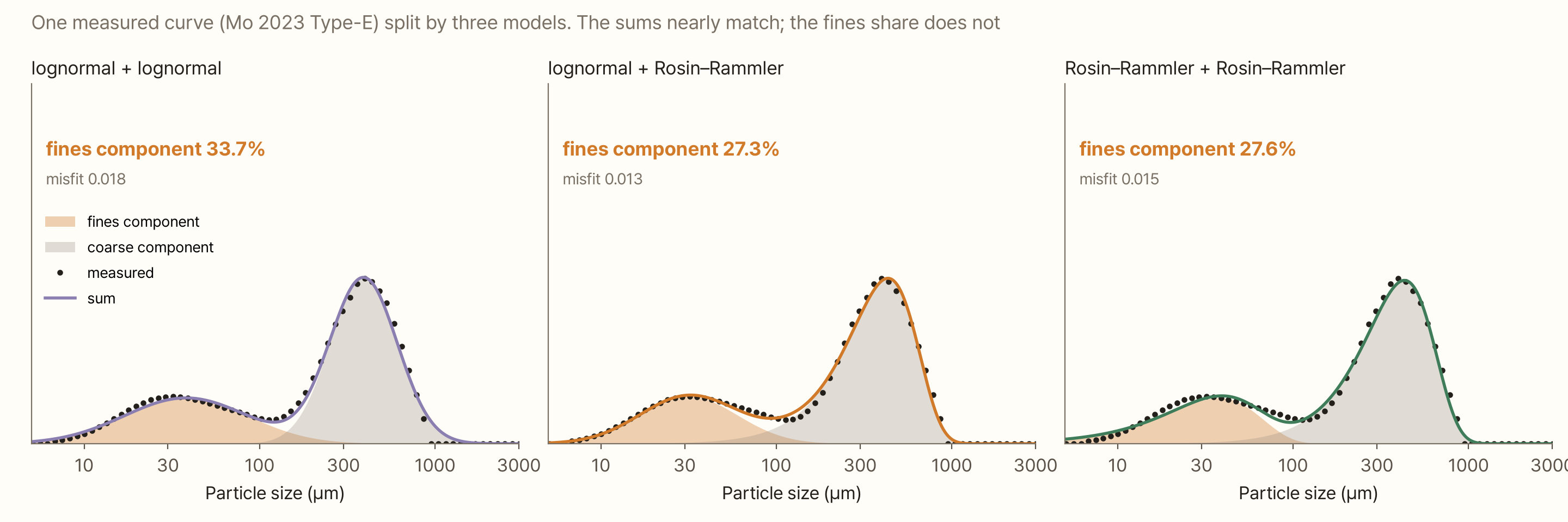
All three models follow the points almost identically. The misfit (root mean square error) is 0.013–0.018, a difference of only about 0.005. But the share of the fines part ranges from 27.3% to 33.7%.

The split happens between the two peaks, from 50 to 200 µm. Which part gets the particles in that range is decided by the shape you choose, not by the data. A lognormal is symmetric on a log scale, so the coarse part has a short left tail, and the fines part spreads out to take what is left over. A Rosin–Rammler has a long left tail on a log scale, so the coarse part takes much of the middle range and the fines part narrows.

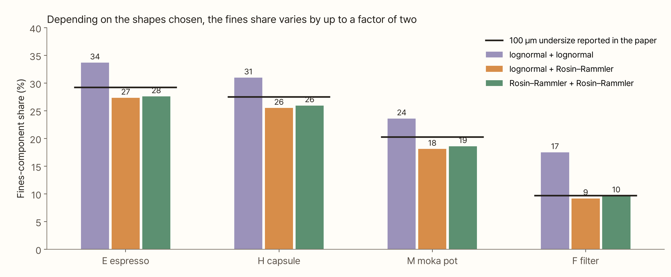
The same thing happened for all four powders. With a lognormal coarse part the fines share always comes out larger; with a Rosin–Rammler coarse part it comes out smaller. For the filter grind F it was 17% versus 9%, a factor of two. It would be nice to pick the model by misfit, but that doesn't work either. The best-fitting model was lognormal + Rosin–Rammler for E and lognormal + lognormal for H, M and F, and the differences were under 0.01.

The 'volume below 100 µm', on the other hand, matched the paper within 1.1 percentage points whichever model it was computed from. What differed between models was the share of the fines part; the curve itself was the same for all of them. A fraction cut at a fixed size comes straight from the data. The share of a part only exists once you assume a shape.

Again, with public raw data

Curves read from a figure always carry some error, so I looked for coffee size distributions with public raw data and repeated the exercise. Méndez Harper et al. (2024) published, under CC BY, the laser-diffraction raw data from their paper on static charge during grinding. There are eight powders: five from bean 1A ground at EK43 setting 2 with 0–20 µL/g of water added before grinding, two from decaf beans at the same setting (a repeat), and one from that decaf powder ground again at setting 6. The instrument was a Mastersizer 2000 (dry), and the volume fractions in all 100 bins are there as measured.

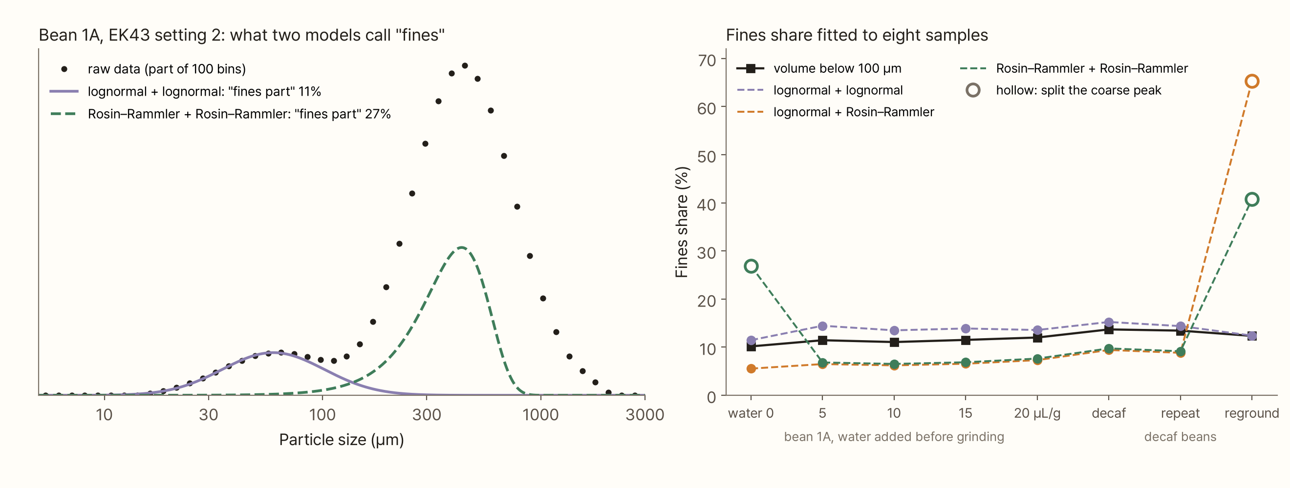
On this data two lognormals fit far better. The misfit was 0.002–0.014, smaller than for the models with a Rosin–Rammler coarse part (0.020–0.032). That is the opposite of Bora and Briesen's result. Even which shape fits best depends on the instrument and the powder.

The fines share split by model again. Two lognormals gave 11–15%; the models with a Rosin–Rammler coarse part mostly gave 6–10%. On the same sample that is a factor of 1.6–2.2. The volume below 100 µm was 10–14%.

The hollow circles deserve a closer look. In two of the eight samples, a model containing a Rosin–Rammler ignored the fines peak and spent its second part on the coarse peak. The green dashed line in the left graph is one of these. It is called the 'fines part', but it is really half of the coarse peak. If the coarse peak's shape differs even slightly from a Rosin–Rammler, patching the misfit of the big peak reduces the error more than fitting the small fines peak, which is only 10% of the total. If you restart the fit near the fines peak you get an answer with a fines share of 6%, but that answer has a larger error. Pick by error alone and the wrong answer wins.

The fitted numbers in Bora and Briesen's supplementary tables show the same tendency. For the 22 samples with clear peaks, the fines share from lognormal + Weibull (10–43%) was larger than from gamma + Weibull by 1.6–7.9 percentage points per sample (median 3.4). The two pairs had almost the same error. Put a heavy-tailed distribution on the fines side and the fines share grows.

One more point. In this raw data the fines peak sits at about 50–65 µm on a log-scale plot, to the right of the 30–40 µm I quoted last time. Instruments use different optical models to turn scattered light into size, and dry dispersion can let fines clumped by static charge into the measurement. Bora and Briesen also write that changing the grind level changes only the height of the fines peak and not its position, so the conclusion that it doesn't move still stands. But when you give its position as a number, you need to say which instrument and which axis.

Fitting again against a known answer

I measured separately how far you drift when you pick the wrong shape. I took the mixture models fitted to the four powders as the 'truth' and refitted those curves with models of other shapes. It amounts to using a mixture distribution as an answer generator.

When the truth was lognormal + Rosin–Rammler, fitting two Rosin–Rammlers recovered the fines share within 0.2 percentage points. With the same coarse shape, a slightly different fines shape does no harm. Fitting the same truth with two lognormals, on the other hand, turned the fines share from 27.3% into 35.0% for E and from 9.2% into 23.1% for F, two and a half times the truth. The misfit in those cases was 0.024–0.029, not very different from the misfit when fitting the measured curves (0.012–0.023). A misfit that size is easy to wave through as 'a good fit'.

Checking with grounds that come with an answer

The answer generator builds its truth from a mixture distribution, so picking a model from the same family as the truth naturally works. Nobody knows what shape real fines have. So I went back to last time's cell-tissue model. In that model every particle carries a label saying where it came from: powder from cells crushed along a crack is the true fines, and pieces split off by cracks are the coarse particles.

I added one thing to the model. Last time's model stopped a piece the moment it became smaller than the gap, so its coarse peak was much sharper than measured. In a real grinder the opening at the burr exit varies from place to place, and the size at which a piece stops depends on where it gets out. So I spread the stopping size for each piece roughly between two thirds and one and a half times the gap (log standard deviation 0.4).

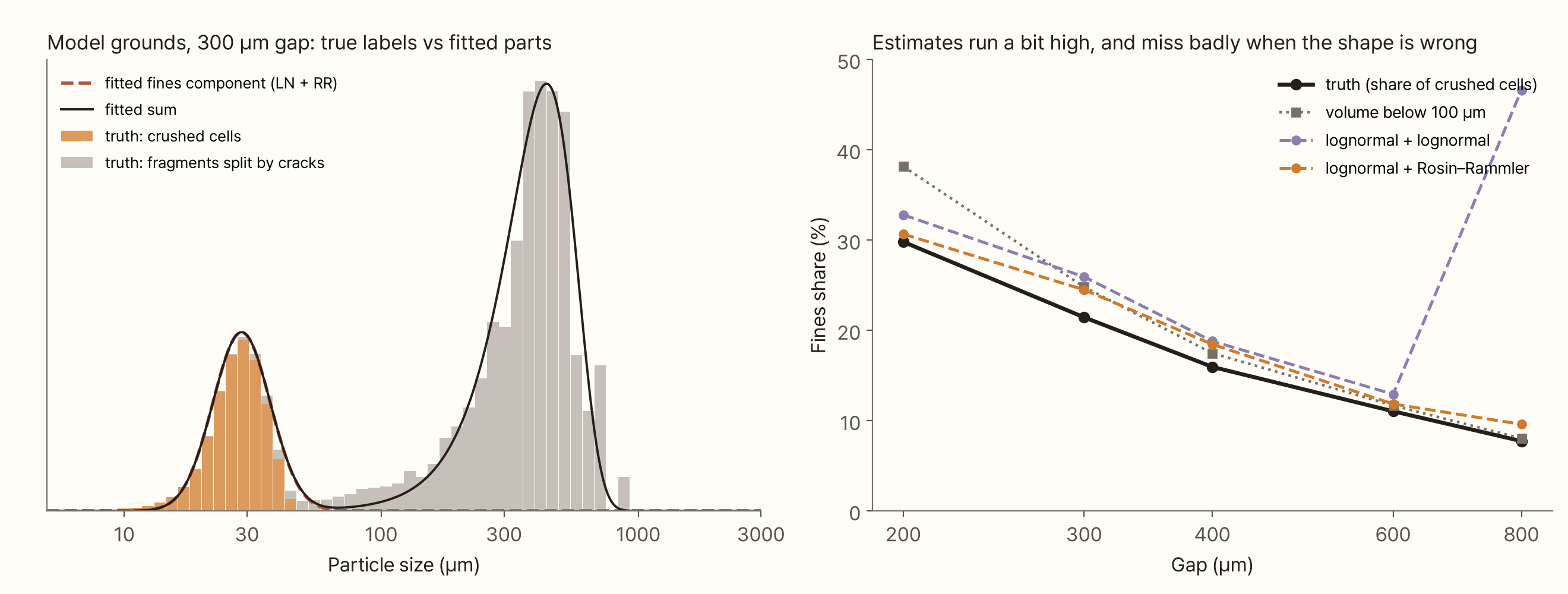
Across gaps of 200–800 µm the true fines share fell from 30% to 8%. The fines share fitted with lognormal + Rosin–Rammler ran 1–3 percentage points above the truth, because the fines part took some of the small pieces between 50 and 150 µm. Two lognormals ran 2–5 points high, and at an 800 µm gap gave 47%. There the model spent its second part not on the fines but on patching the lopsided shape of the coarse peak. The number looks plausible; what it describes is nonsense.

The 'volume below 100 µm' came out above the truth when the gap was narrow (38% against 30% at 200 µm), because at fine settings the coarse pieces themselves reach down to around 100 µm. For gaps wider than 400 µm it was within 2 points of the truth.

In short, the mixture model with a Rosin–Rammler coarse part estimated the amount of fines a little high but consistently. That points the same way as Bora and Briesen's finding that Weibull fits the coarse part of real grounds, though the raw data above preferred a lognormal. This is a result inside my model. There is no guarantee real fines have the same shape as the model's.

When you can't see the small end

The measuring tool in Part 1 was a camera, and a camera barely sees fines. Can a mixture model still estimate them? I deleted everything below a given size from the measured Type-E curve and fitted.

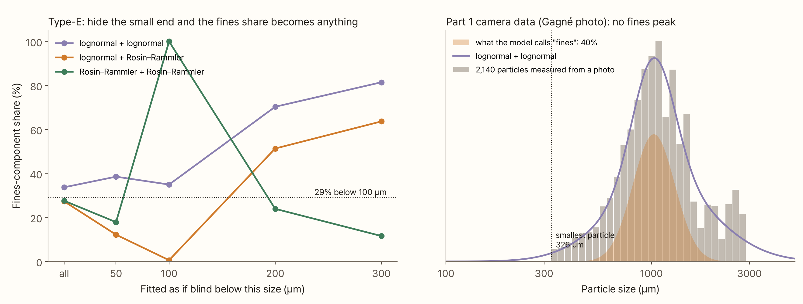
As the left graph shows, hiding the small end up to just 50 µm scatters the fines share from 12% to 39%. Hiding everything below 100 µm gives 0.6%, 35% or 100% depending on the model. Hiding everything below 200–300 µm gives 12–81%, and the 'fines part' is then not fines at all but one half of a split coarse peak.

On the right are the 2,140 particles measured in Part 1 from Gagné's photo. The smallest is 326 µm, so there is no fines peak at all. Fit mixture models to it and two lognormals call 40% 'fines', while the two models with a Rosin–Rammler call 86–87% 'fines'. Either way they have just split the large particles near 1,000 µm in two. A model can't find a peak that isn't in the data.

A Rosin–Rammler straight line through the same photo data gives n of 3.0 and R² of 0.95. That looks like a much more even powder than the laser-measured grounds (n of 1.1). A measurement that can't see fines makes a powder look more even than it is. From Part 1's photo measurements you can only talk about the large-particle side, the shape of the coarse part.

Try it yourself

Below you can pick data and models and fit them yourself. Choose the data with the buttons at the top. Measured E·H·M·F are the curves read from Mo et al. (2023); 'raw data' are two EK43 powders from Méndez Harper et al. (2024); 'model grounds' are the cell-tissue model with true labels; the 'answer generator' makes a curve from fines and coarse parts set with sliders; 'Part 1 camera' is the particles measured from Gagné's photo. Pick a model on the right and it fits at once. Orange is the fines part, grey the coarse part, and where the answer is known, a red dotted line shows the true fines. Raise 'blind below' to mimic an instrument that can't see the small end.

In the answer generator, widen the fines or lower the coarse evenness (n) and the two peaks overlap. Then watch how far apart the fines shares of the three models in the table below drift.

What this conclusion leaves out

• Mo et al.'s curves are values read from a figure. The volume below 100 µm matched the paper within 0.6 points, but d[3,2] came out 5% low; the very small tail was under-read. Refitting the original data could shift the numbers a little
• I only looked at three model families. Bora and Briesen (2026) compared ten. Other shapes such as gamma or beta-prime would shift the fines share again
• I used only one fitting criterion. I minimised the squared error of the density per log size. Bora and Briesen minimised the error of the density on a µm axis. Fitting the cumulative curve or weighting bins differently changes the result. This difference may be part of why the best shape differs between this piece and their results
• The raw data cover one grinder and one setting. Méndez Harper et al.'s data are EK43 setting 2 only (plus one regrind), and being dry measurements, they may include fines clumped by static charge
• The grounds with an answer come from a 2D model. The result that the fines part runs 1–3 points above the truth depends on the shape of this model's fines. Real fines also contain wall fragments much smaller than a cell and oil droplets, so they spread wider
• The gap spread (0.4) is a value I chose. I found no measurement of how widely the size at which pieces leave a real burr exit varies
• The camera data come from different beans. Gagné's photo and Mo et al.'s powders are not the same coffee, so their n can't be compared directly. I used it only as an example of how much the measuring method changes the apparent evenness

Summary

• The classic distributions of comminution theory (Rosin–Rammler, lognormal) have one peak. Fitted to coffee grounds they follow only the large peak; for the espresso grind they captured 11% (Rosin–Rammler) and 2% (lognormal) of the 30% below 100 µm
• On Rosin–Rammler paper, R² stays high at 0.93–0.95 even when the fines are missed. The evenness n came out as 1.1 from a straight-line fit and 1.5–2.0 from a density fit
• There are two peaks because two lengths set the sizes. Pieces follow the gap; cells that come loose follow the cell size. In mineral comminution, splitting and abrasion together produce a similar two-peaked distribution
• Five-number mixture models follow the curve well, but the fines-part share split with the chosen shapes: 27–34% for the espresso grind and 9–17% for the filter grind. On public raw data (EK43) it split into 11–15% and 6–10%. Misfit couldn't decide between them, and in two of the eight raw-data samples the lowest-error answer was a wrong one that split the coarse peak
• On model grounds with a known answer, the model with a Rosin–Rammler coarse part estimated the fines share 1–3 points high, but consistently. Two lognormals drifted further and once called the wrong thing fines
• If you can't see the small end, the fines share can come out as anything. Part 1's photo measurements have no fines peak, so a mixture model just splits the large particles in two

If you want to say how much fines there are, pick one of two routes. A fraction below a fixed size (such as the volume below 100 µm) comes straight from the data without a model. If you use the fines part of a mixture model, report which shapes you chose along with it. Both only hold for data from an instrument that can see the fines peak.

References

• Rosin P, Rammler E (1933). The laws governing the fineness of powdered coal. Journal of the Institute of Fuel 7, 29–36 — original not seen; citation and formula only
• Weibull W (1951). A statistical distribution function of wide applicability. Journal of Applied Mechanics 18, 293–297
• Bora M, Briesen H (2026). Characterization of bimodal particle size distribution of ground coffee powder. Journal of Food Process Engineering 49(6), e70645. doi:10.1111/jfpe.70645
• Khongphinitbunjong K, Wongsakul S, Mookum T (2025). Particle size distribution model for optimizing coffee grind consistency. Journal of Food Process Engineering 48(5), e70129. doi:10.1111/jfpe.70129
• Méndez Harper J, McDonald CS, Rheingold EJ et al., Hendon CH (2024). Moisture-controlled triboelectrification during coffee grinding. Matter 7, 266–283. doi:10.1016/j.matt.2023.11.005 — laser-diffraction raw data: figshare doi:10.6084/m9.figshare.23277320 (CC BY 4.0)
• Petrakis E (2023). Effect of size-distribution environment on breakage parameters using closed-cycle grinding tests. Materials 16(24), 7687. doi:10.3390/ma16247687 — Austin-type two-term breakage function
• Austin LG, Luckie PT (1972). Methods for determination of breakage distribution parameters. Powder Technology 5(4), 215–222. doi:10.1016/0032-5910(72)80022-680022-6)
• Mair K, Abe S (2011). Breaking up: comminution mechanisms in sheared simulated fault gouge. Pure and Applied Geophysics 168, 2277–2288. doi:10.1007/s00024-011-0266-6
• Mo C, Johnston R, Navarini L, Suggi Liverani F, Ellero M (2023). Exploring the link between coffee matrix microstructure and flow properties using combined X-ray microtomography and smoothed particle hydrodynamics simulations. Scientific Reports 13, 16374. doi:10.1038/s41598-023-42380-y — the four distributions in Fig. 3, Table 1
• Gagné J. coffeegrindsize. GitHub. link — the example photo used in Part 1

Image credits

• All graphs, the cover and the simulation: my own
• Measured curves: read from Fig. 3(a) of Mo C et al. (2023), Scientific Reports 13:16374, and redrawn. CC BY 4.0
• Raw-data graphs: drawn from the public figshare data of Méndez Harper et al. (2024) (CC BY 4.0)
• Part 1 camera data: particles measured in "What Is a Diameter?" from the example photo in Jonathan Gagné's coffeegrindsize (MIT licence)