The Size of a Single Pixel
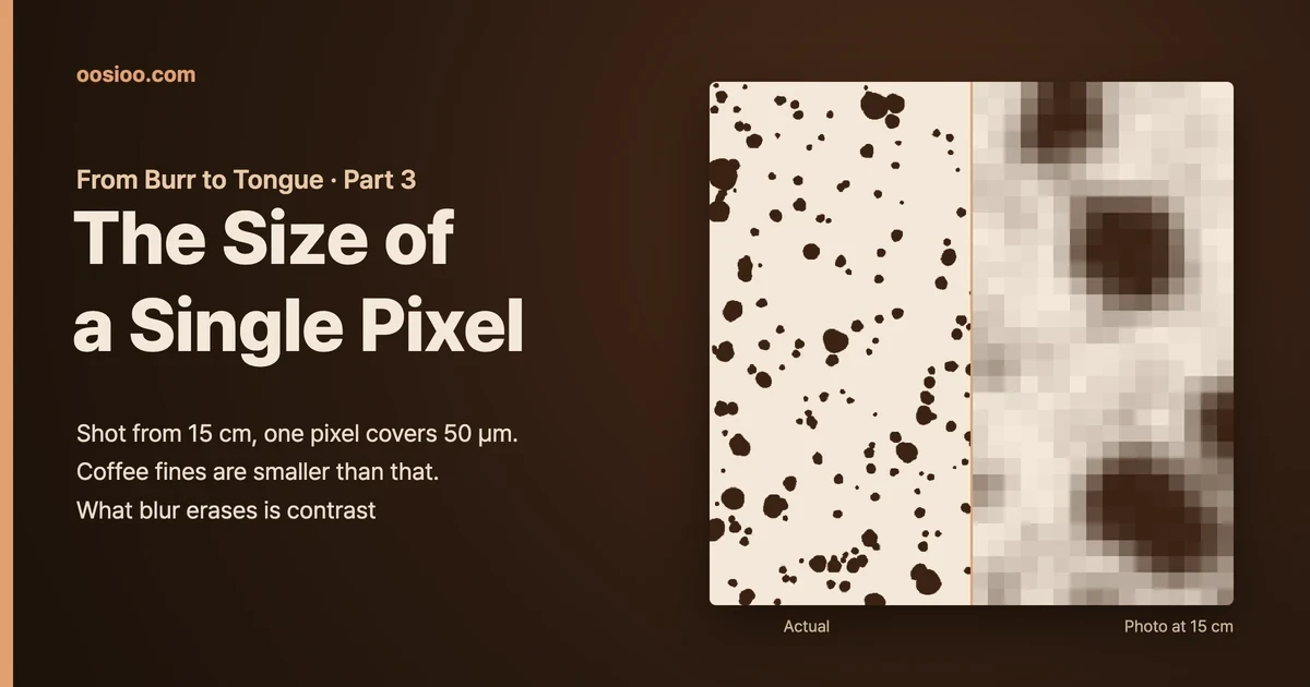
Hold a phone 15 cm above the paper and one pixel covers about 50 µm, while coffee fines peak at 30–40 µm. Following a single particle through lens blur, pixels, noise and a brightness cutoff in synthetic photos shows that, with 0.8 px of blur, particles under about 96 µm vanish entirely and measuring size within ±5% takes a diameter of 8–10 pixels. Photograph a virtual sample that is 20% fines by volume, and the fines shrink to 0.1%.
The last two pieces were about getting the photo's scale right. Swapping the coin for four markers and flattening the photo shrank the error from camera tilt to around 0.1 percentage points. The biggest error left was the printer's "fit to page" setting, and a single card was enough to check for it. We now know fairly precisely how many pixels 1 mm takes up in a photo.
But Part 1 mentioned one number in passing. Hold a phone 15 cm above the paper and one pixel covers about 50 µm of it. Coffee fines peak at around 30–40 µm. In other words, a single fine is smaller than a single pixel.
So what happens to a particle smaller than a pixel? You might expect it to vanish, but that's not quite right. A small particle still blocks some light, so the pixel where it sits gets a little darker. The real questions are whether you can look at that darker pixel and call it a particle, and, if you can, how accurately you can measure its size. This piece follows a single particle on its way to becoming pixels and works out how many pixels it needs before its size can be trusted.
The Rooms Hooke Saw in Cork
In 1665, the English scientist Robert Hooke published Micrographia, a book of drawings of what he saw through microscopes he built himself. One of its plates shows a thin slice of cork. Hooke noticed that cork was divided into tiny rooms, like a honeycomb, and called them "cells." That is where the biological word comes from.
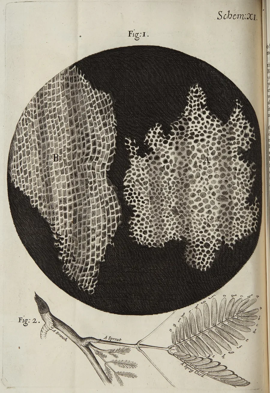
Robert Hooke, Micrographia (1665), Plate XI. The two upper drawings are cork sections. Image: Robert Hooke / Wikimedia Commons (public domain)
A coffee bean is a plant seed, so it is built the same way. Cut a roasted bean open and you find small rooms walled off by cell walls, packed tightly together. Mo et al. (2023) looked inside coffee grounds with X-ray tomography and reported that the bean's cells are 25–50 µm in size. They explained that the small peak that commonly shows up in the particle size distribution of ground coffee, the particles around 30–40 µm usually called fines, consists of cell-wall fragments. That is why the fines peak lands in a similar place no matter how different the grinders are. The size of the fines is set by the bean's cells, not by the grinder.
Hooke built a microscope to see things at this scale. We're trying to measure them with a phone.
The Grid from 15 cm Up
Let's reuse the camera model from Part 1: a phone main camera with a 4032×3024-pixel image and a 26 mm-equivalent lens. With this camera, the size one pixel covers on the paper grows in proportion to the camera's height.
| Phone height | One pixel | 35 µm fine | 100 µm particle | 400 µm particle |
|---|---|---|---|---|
| 30 cm | 99 µm | 0.35 px | 1.0 px | 4.0 px |
| 15 cm | 50 µm | 0.71 px | 2.0 px | 8.1 px |
| 10 cm | 33 µm | 1.1 px | 3.0 px | 12 px |
| 5 cm | 17 µm | 2.1 px | 6.1 px | 24 px |
Calculated with the pinhole model from Part 1. "px" is how many pixels the particle's diameter spans in the photo
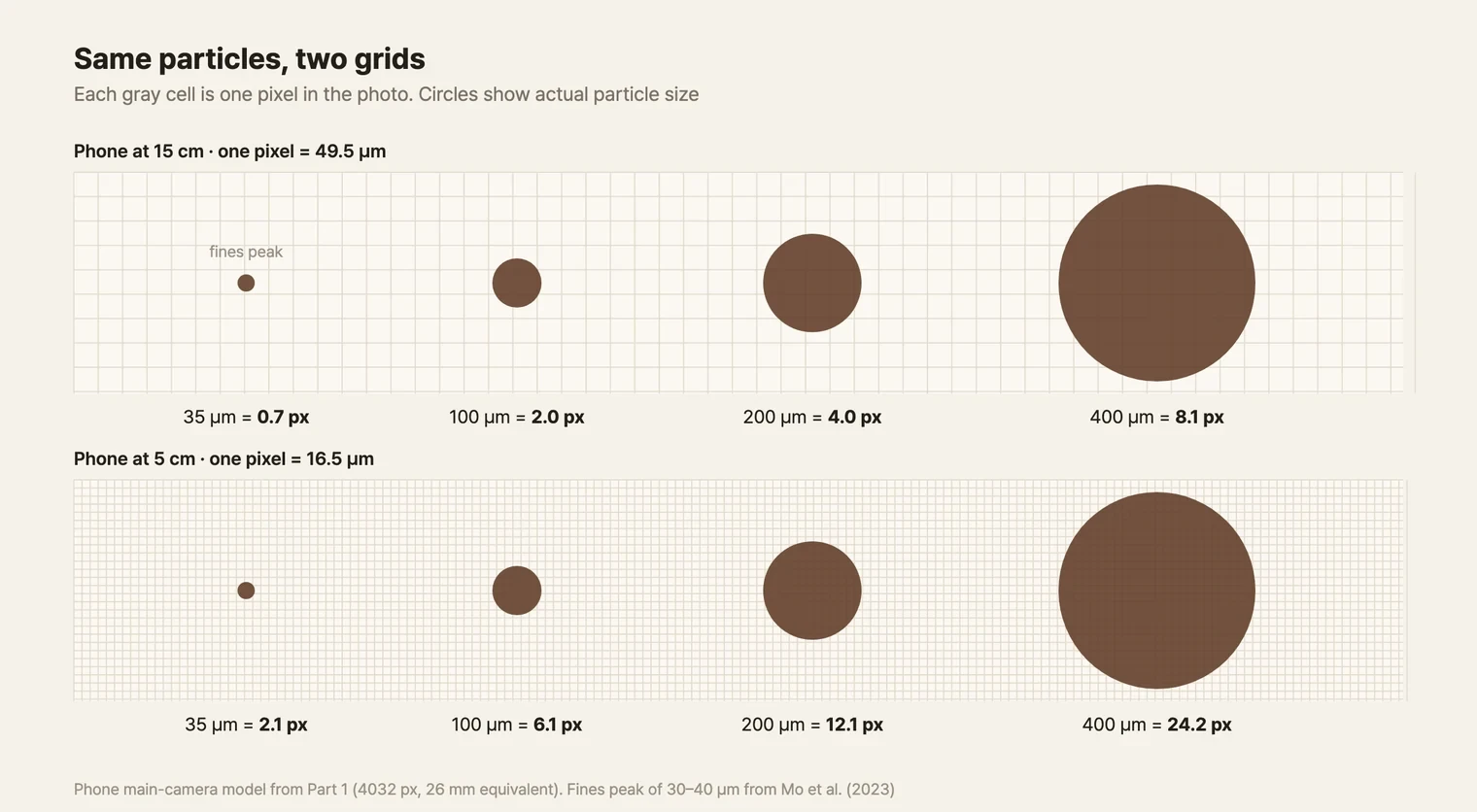
Unspecialty's column scaled its flattened photos so that one pixel equals 27.5 µm. In this camera model, that corresponds to a height of a little over 8 cm. Even at that scale, a 100 µm particle is 3.6 pixels across.
A particle 2 pixels across covers an area of a little over 3 pixels. Depending on where it lands on the pixel grid, it might straddle four pixels a little each, or nearly fill one pixel and spill slightly into its neighbors. The same particle gets recorded differently just by sitting in a different spot. Blur comes on top of that.
The Lens Blurs First
Light spreads out when it passes through the opening of a lens. Even a perfectly made lens can't record a point as a point. It records a small disc, bright in the middle and surrounded by faint rings. This is called the Airy disk. Its size is set by the wavelength of the light and the aperture (f-number).
When two points are too close, their disks overlap and look like one. Lord Rayleigh took the distance at which the center of one disk falls on the first dark ring of the other as the limit for just barely telling two points apart (Rayleigh 1879). Optics still uses this criterion to talk about resolution.
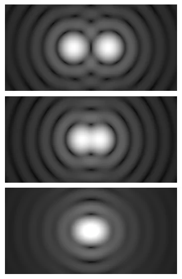
Airy disks of two points moving closer together. The middle row is the Rayleigh criterion. Image: Spencer Bliven / Wikimedia Commons (public domain)
Let's apply this to a phone's main camera. Take the iPhone 14 Pro: its main camera has an f/1.78 aperture (Apple), and it combines four pixels of its 48-megapixel sensor to work like a single 2.44 µm pixel (Apple 2022). I plugged these two values into the camera model from Part 1. In green light (0.55 µm), the Airy disk is 2.44 × 0.55 µm × 1.78 ≈ 2.4 µm across, nearly the same as one combined pixel. Holding this camera model 15 cm up and converting to the paper side, the Rayleigh limit comes to about 24 µm and the disk to about 49 µm across, roughly one pixel (49.5 µm) (model estimate).
Making pixels much smaller than the disk the lens draws only slices the same blurry disk into finer pieces. Shoot at 48 megapixels and the pixels halve (1.22 µm), but the disk stays the same, so one disk spans two pixels. Four times the pixel count does not mean four times the resolution.
Diffraction is only where the blur starts. Real photos pile on several more layers.
- Lens aberrations. Real lenses fall short of the diffraction limit, more so toward the edges of the frame
- Shake. A handheld phone moves slightly during the exposure. Stabilization catches most of it, but not all
- Demosaicing. Each pixel on a phone sensor receives only one of red, green or blue. The other two colors are borrowed from neighboring pixels to fill in
- Compression and processing. Saving as JPEG or HEIF smears fine detail, and the phone also sharpens edges to make the photo look crisp
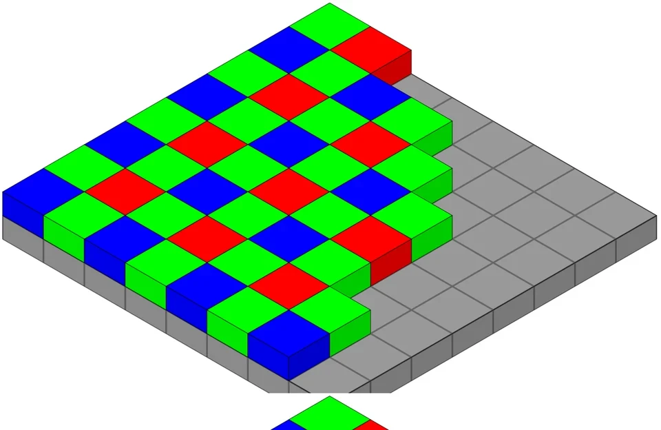
A Bayer filter. Each pixel receives a single color, and green takes up half (Bayer 1976). Image: Cburnett / Wikimedia Commons (CC BY-SA 3.0)
How much blur all of this adds up to varies by camera and by how you shoot, and no figures are published. In this piece I model the total blur as a Gaussian with a standard deviation σ of 0.5–1.0 pixels and use 0.8 pixels as the baseline. The real value has to be measured. The standard way to measure a digital camera's resolution is to photograph a slightly slanted black edge and see how far it spreads (ISO 12233). Conveniently, the marker sheet already has edges like that: the black borders of the markers.
How a Particle Becomes Pixels
Now let's photograph one particle. As in the last piece, I build a synthetic photo where the right answer is known. Put the particles on a bright panel such as a light pad and light them from below, and each particle becomes a dark shadow on a bright background. I set the background brightness to 1 and the particle to 0.
There are five steps. Draw the actual particle shape very finely, add blur, average it into pixel-sized blocks, and mix noise into each pixel (2% of brightness). Finally, call every pixel darker than 0.5 a particle pixel. The diameter of a circle with the same area as those pixels is the measured diameter.
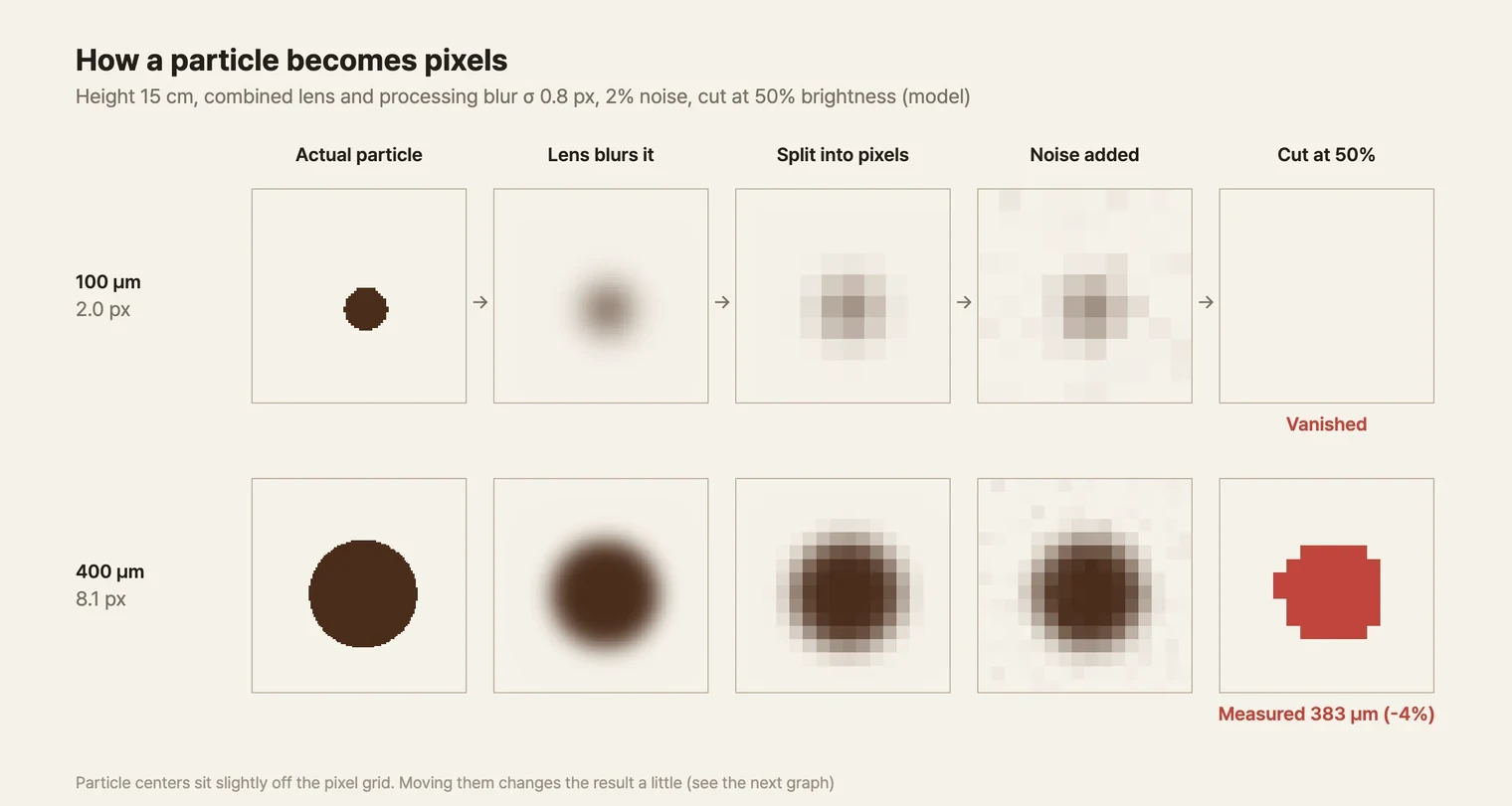
Blur σ 0.8 px. All calculations are my own for this series
As the 100 µm particle blurs, even its center ends up brighter than 0.5. The pixels where it sits clearly got darker, but they don't cross the cutoff, so the particle drops out of the result entirely. The 400 µm particle is detected, and its measured diameter comes out a little small.
The size below which a particle vanishes entirely is easy to work out. Blur a disc with a Gaussian, and its center brightness is exactly 0.5 when the diameter d equals 2.355σ. Any smaller particle never gets darker than 0.5, even at its darkest point. With 0.8 pixels of blur, that's a diameter of 1.9 pixels, or about 96 µm at a height of 15 cm. With 0.5 pixels of blur it's 61 µm; with 1.0 pixel, 118 µm. It isn't that a pixel can't hold a particle this small. It's that blur wipes out a small particle's contrast.
How Many Pixels Before You Can Trust the Size?
I shifted the particle slightly across the pixel grid and measured each size 200 times. In the graph below, the line is the average of measured diameter divided by actual diameter, and the band is the range that 95% of the 200 measurements fell into.
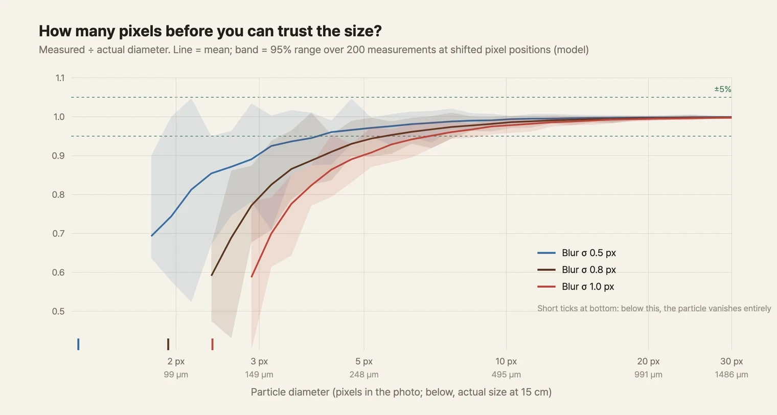
Blur σ is assumed to combine lens, shake and processing. All calculations are my own for this series (model estimate)
Reading off the 0.8-pixel blur:
- A particle 3 pixels across (150 µm at 15 cm) is measured 20% small on average
- 4 pixels (200 µm) comes out 10% small, 6 pixels (300 µm) 4%, and 10 pixels (500 µm) 1.3%
- For the 95% range to fall within ±5%, the diameter needs to be 8–10 pixels: 400–500 µm at 15 cm
There's a reason small particles get measured small. A straight edge, even when blurred, keeps its 0.5-brightness line right where the original edge was, because the same amount spreads to each side. But a circle's edge is curved. On the inside, the particle wraps around the edge; on the outside, the background wraps around it. So when it blurs, more of the bright background mixes inward. The 0.5 line gets pushed inward, and the smaller the circle, the more sharply its edge curves and the farther the line is pushed. A 4-pixel circle shrinking by 10% and a circle of just over 2 pixels vanishing altogether are the same effect.
The 95% range comes from where the particle sits on the grid. Even for the same 4-pixel particle, the number of pixels that pass the cutoff changes by a few depending on how it straddles pixel boundaries. For a large particle, a few pixels are small next to its total area. For a small particle, those few pixels are a large share of it.
Changing the Cutoff Brightness
If the trouble is that small particles vanish, why not move the cutoff toward the background? Count every pixel darker than 0.7 instead of 0.5 as particle, and blurred small particles get picked up too.
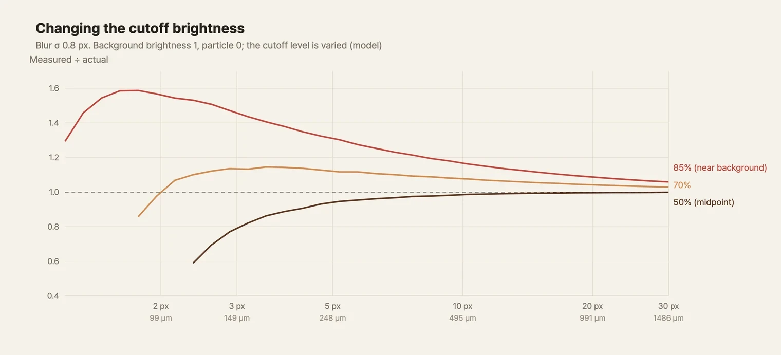
Blur σ 0.8 px. All calculations are my own for this series (model estimate)
At 0.7, particles 2 pixels across (100 µm) start to get detected. In exchange, every particle grows. A 2-pixel particle is measured about right on average, but its 95% range widens from −20% to +13%. Particles of 3–4 pixels come out 13–14% large, 10 pixels 7.6% large, and even 20 pixels 4.2% large. At 0.85, about 40% of 1-pixel particles get detected, but a 10-pixel particle grows by 17%.
This time even straight edges move. Set the cutoff away from 0.5 and the edge shifts outward by an amount proportional to the width of the blur. That distance is fixed in pixels regardless of particle size, so the smaller the particle, the more it swells.
In the end, no single cutoff rescues small particles while measuring large ones accurately. Knowing the blur width changes things. If you know the blur, you can fit each particle with a model, "a disc this size blurred this much gets recorded like this," and work backward to its size. To do that, you first have to measure the blur in that photo. The marker borders mentioned above can do that job.
Moving Closer
What if you shoot from closer? Drop to 5 cm and one pixel becomes 17 µm, so a 100 µm particle spans 6 pixels. But it isn't free.
A camera focuses exactly at only one height. A point away from that height spreads into a blur circle whose size is proportional to the diameter of the lens opening (the entrance pupil) and inversely proportional to the distance from the camera. Working out the height range where the blur circle stays within one pixel gives ±1.8 mm at 15 cm, ±0.8 mm at 10 cm and ±0.2 mm at 5 cm (model estimate).
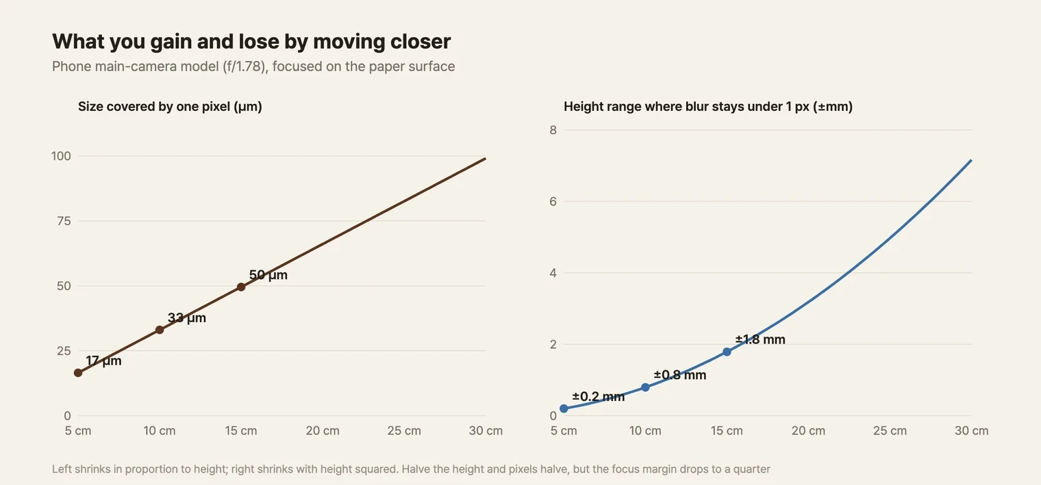
Pixel size shrinks in proportion to height, but the range of heights in focus shrinks with the square of height. Halve the height and the pixels halve, but the focus margin drops to a quarter. At half the distance the blur circle doubles while the pixel halves, so the blur measured in pixels quadruples.
±0.2 mm is very tight for coffee grounds. Coarse particles are hundreds of µm thick, so their tops and bottoms can't both be in focus at once. With backlighting you see each particle's shadow outline, and the height at which that outline forms differs from particle to particle. Even a slight ripple in the paper pushes it out of focus. And if you switch on macro mode to get closer still, you end up shooting with the ultra-wide camera, which, as we saw in Part 1, has the most distortion.
15 cm is roomy. Even if focus is off by 1 mm, the blur circle is 0.6 pixels, and in the earlier calculation the measurement of a 4-pixel particle barely changed (0.905 → 0.902). You give up resolution and buy slack in focus and distortion in return.
How the Missing Fines Change the Distribution
So far we've looked at one particle at a time. Now let's look at a handful of coffee. Before grinding and photographing real coffee, I built a virtual ground sample where the right answer is known: a bimodal distribution with 20% of the volume in fines (median 35 µm) and 80% in coarse particles (median 500 µm). A 20% fines volume falls within the 9.7–29.2% that Mo et al. (2023) measured by laser diffraction as the volume fraction under 100 µm in four coffees.
First, a surprising number. Fines that make up 20% of the volume make up 99.8% of the particles by count. A particle 14 times smaller in diameter has about 2,900 times less volume, so it takes that many more of them to fill the same volume. Count a handful of ground coffee particle by particle and nearly all of it is fines.
I photographed this sample with the model above.
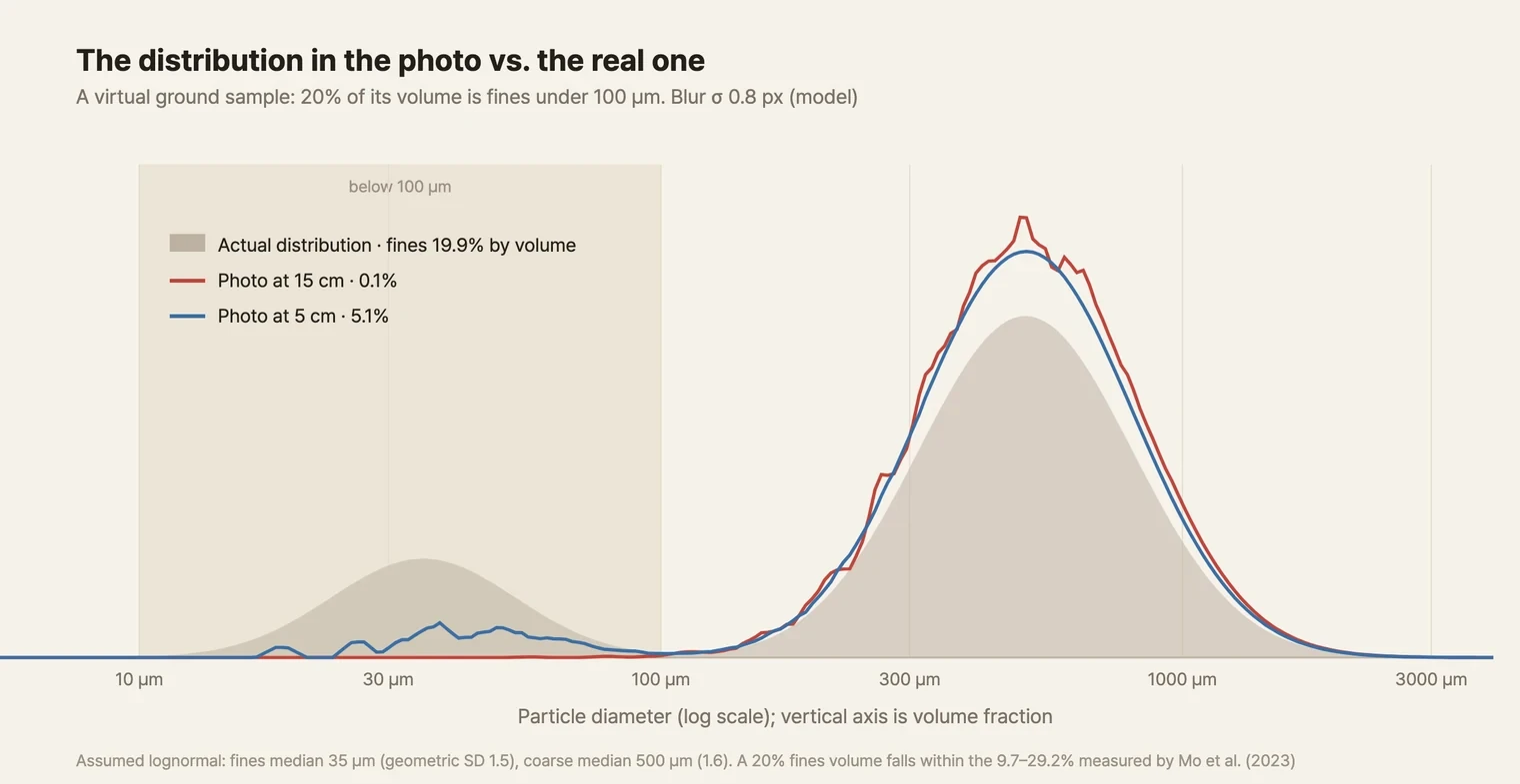
Blur σ 0.8 px. All calculations are my own for this series (model estimate)
In the distribution measured from the photo taken at 15 cm, the volume under 100 µm was 0.1%. Nearly all of the actual 20% disappeared. By count, only 2 particles in 1,000 were detected. Reducing the blur to 0.5 pixels only brings it to 0.3%. Dropping to 5 cm raises it to 5.1% (10.4% with 0.5 pixels of blur), still only about a quarter of the real value.
The missing fines change other numbers too. A distribution is always drawn to add up to 100%, so when the fines drop out, the coarse particles' share grows by the same amount. The volume-weighted median diameter went from an actual 425 µm to 502 µm measured from the 15 cm photo, 18% coarser.
Below is a 3×2 mm close-up of the same virtual sample.
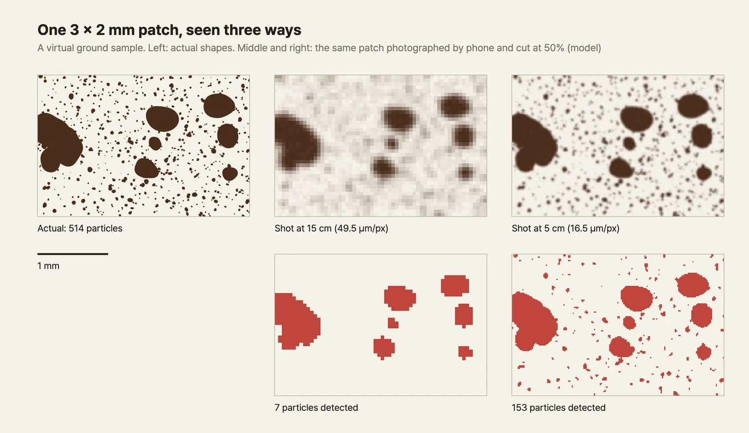
Particle shapes are circles distorted slightly at random. All calculations are my own for this series
This 3×2 mm patch holds 514 separate particles. In the 15 cm photo, 7 were detected as particles, all of them coarse. Six of those swallowed neighboring fines and became clumps larger than the real particle. In the 5 cm photo, 153 were detected. 132 matched a single particle, but 21 were two or more particles stuck together by blur. All the detections together cover only a third of the actual particles (178).
In the 15 cm photo the fines didn't disappear. They remain as patches where the background is slightly darker. Add up the brightness of the whole photo and the amount of light those fines blocked is in there too. They just can't be caught as individual particles. That difference matters. Even if you can't count them one by one, there's still a way open to estimate the amount of fines from how much darker the background is than usual. I haven't tried it yet.
Try It Yourself
In the simulation below you can change the phone height, blur, cutoff brightness and noise. On the left, five particles from 35 to 400 µm are magnified at the same scale as they would be photographed. The blue dashed circle is the actual particle, and the red cells are pixels judged to be particle. On the right are the results of photographing particles from 20 to 1000 µm, 40 times at each size. Click the left panel to reshuffle where the particles sit.
What This Model Leaves Out
These calculations are meant to give a feel for how bad the measurement can get. Real photos contain plenty that the model doesn't.
- The actual blur. σ of 0.5–1.0 pixels is an assumption. It will differ between phones and between the center and edges of the frame
- Sharpening. Phones emphasize edges to make photos look crisp, which adds a bright fringe outside an edge and darkens the inside. This processing can shift an edge cut at 0.5 in either direction. Shooting RAW avoids much of it
- Particle shape. Real coffee particles aren't discs, and they have thickness. The problems shape causes are big enough to deserve their own treatment
- Particles touching. Blur joins two nearby particles into one. You can see this in a few places in the 3×2 mm figure above
Still, the direction of the conclusion doesn't change. A handheld phone photo can measure the distribution of coarse particles, but it can't count fines particle by particle. A measurement result needs the caveat "distribution of particles larger than so many µm." A distribution drawn without that caveat looks like coffee with no fines.
Summary
- Hold a phone's main camera 15 cm up and one pixel covers about 50 µm. The fines peak (30–40 µm) comes from the size of the bean's cells and is smaller than one pixel
- Diffraction from the lens alone makes an Airy disk about one pixel across. Aberrations, shake, demosaicing and compression add more blur on top
- A blurred disc drops out of the result entirely once its center brightness rises above 0.5. With 0.8 pixels of blur, particles under 1.9 pixels across, about 96 µm at 15 cm, vanish
- Particles that are detected still measure smaller the smaller they are, because blurred curved edges get pushed inward. Staying within ±5% takes a diameter of 8–10 pixels (400–500 µm at 15 cm)
- Moving the cutoff toward the background rescues small particles but swells every particle. No single cutoff gets both right
- Moving closer shrinks pixels in proportion to height, but the focus margin shrinks with height squared. At 5 cm it's ±0.2 mm
- Photograph a virtual sample whose volume is 20% fines from 15 cm and the fines shrink to 0.1%, while the volume-weighted median diameter comes out 18% coarser
Parts 1 and 2 were about checking whether the marks on our ruler were right. This time we asked what the smallest thing that ruler can measure is. Measuring coffee with a phone was always going to mean seeing only part of the coffee. What matters is knowing which part you're looking at.
References
- Hooke R (1665). Micrographia. London: Martyn and Allestry. doi:10.5962/bhl.title.904 — Observation XVIII (cork) and Plate XI, bibliographic reference verified
- Mo C, Johnston R, Navarini L, Liverani F, Ellero M (2023). Exploring the link between coffee matrix microstructure and flow properties using combined X-ray microtomography and smoothed particle hydrodynamics simulations. Scientific Reports 13, 16374. doi:10.1038/s41598-023-42380-y — cell size 25–50 µm, fines peak 30–40 µm, volume fraction under 100 µm 9.7–29.2%
- Rayleigh, Lord (1879). Investigations in optics, with special reference to the spectroscope. Philosophical Magazine 8(49), 261–274. doi:10.1080/14786447908639684 — Rayleigh criterion, bibliographic reference verified
- Bayer BE (1976). Color imaging array. US Patent 3,971,065 — the Bayer filter
- Apple (2022). Apple debuts iPhone 14 Pro and iPhone 14 Pro Max. Link — 2.44 µm quad pixel verified
- Apple. iPhone 14 Pro - Technical Specifications. Link — main camera 24 mm, f/1.78 verified
- ISO 12233:2023. Photography — Electronic still picture imaging — Resolution and spatial frequency responses — measuring resolution with a slanted edge
- Unspecialty (2023). "Developing a Grind-Size Guide." Link — 27.5 µm/px
Image Credits
- Micrographia Plate XI: Robert Hooke (1665), Wikimedia Commons, public domain
- Rayleigh criterion: Spencer Bliven, Wikimedia Commons, public domain
- Bayer filter: Cburnett, Wikimedia Commons, CC BY-SA 3.0 (SVG converted to PNG)
- All other figures, synthetic photos and simulations: created by the author


